Green Bay Packers vs Cleveland Browns Match Player Stats
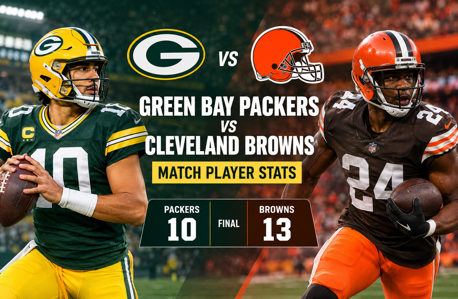
The green bay packers vs cleveland browns match player stats from September 21, 2025, tell the story of a close NFL contest decided by a dramatic fourth-quarter turnaround. The Cleveland Browns defeated the Green Bay Packers 13-10, scoring all 13 of their points in the final quarter after neither team managed to score in the first quarter. Green Bay entered the fourth quarter with a 10-0 lead, but Cleveland’s rushing attack, defensive pressure, and late scoring opportunities changed the outcome. Quinshon Judkins led the Browns on the ground with 94 rushing yards and a touchdown, while Jordan Love passed for 183 yards and one touchdown for Green Bay. The final box score highlights how defensive execution, rushing efficiency, and red-zone opportunities can matter more than total passing yards in a tightly contested football game.
Green Bay Packers vs Cleveland Browns Match Player Stats: Game Overview
The Week 3 matchup took place on September 21, 2025. Cleveland secured a three-point victory, improving its overall record to 1-2, while Green Bay fell to 2-1.
Cleveland Browns
Home team · Record after game: 1-2
13 points
Green Bay Packers
Away team · Record after game: 2-1
10 points
Game date
September 21, 2025
Final result
Browns won by 3
Competition
NFL regular season
Game status
Final
Final score by quarter
| Quarter | Green Bay Packers | Cleveland Browns |
| First | 0 | 0 |
| Second | 3 | 0 |
| Third | 7 | 0 |
| Fourth | 0 | 13 |
| Final | 10 | 13 |
The quarter-by-quarter scoring reveals the central feature of this game. Green Bay scored a field goal in the second quarter and a touchdown in the third. Cleveland then scored 13 unanswered points in the fourth quarter to complete the comeback.
This scoring pattern matters because it shows that the Browns did not need to dominate the entire game. They needed to improve their offensive production late, maintain defensive pressure, and convert enough opportunities to move ahead.
The supplied ESPN box score is the primary data source for the player statistics and final result discussed below.
Quarterback Stats: Jordan Love vs Joe Flacco
Quarterback production is one of the most important parts of any NFL box score, but passing yards alone do not explain how a game unfolds. This matchup provides a useful example of the difference between efficient passing and converting that efficiency into points.
Jordan Love’s passing performance
| Statistic | Jordan Love |
| Completions | 18 |
| Pass attempts | 25 |
| Completion percentage | 72.0% |
| Passing yards | 183 |
| Yards per attempt | 7.3 |
| Passing touchdowns | 1 |
| Interceptions | 1 |
| Sacks taken | 5 |
| Yards lost to sacks | 34 |
| Passer rating | 89.2 |
| ESPN QBR | 56.4 |
Love completed 18 of his 25 passes, giving him a 72% completion rate. His 183 passing yards and 7.3 yards per attempt indicate that he was able to move the ball through the air at a reasonable rate.
His touchdown pass to tight end John FitzPatrick gave Green Bay its only offensive touchdown. The scoring play, a three-yard completion in the third quarter, extended the Packers’ lead to 10-0.
However, Love’s five sacks and one interception were significant. Sacks can turn manageable situations into long-yardage downs, disrupt offensive rhythm, and force a team to settle for field goals or punts. An interception in a close game can be even more costly when it gives an opponent a short field.
That is exactly why the final result deserves more attention than the passing totals alone. Love’s completion percentage was strong, but Green Bay could not preserve its lead.
Joe Flacco’s passing performance
| Statistic | Joe Flacco |
| Completions | 21 |
| Pass attempts | 36 |
| Completion percentage | 58.3% |
| Passing yards | 142 |
| Yards per attempt | 3.9 |
| Passing touchdowns | 0 |
| Interceptions | 1 |
| Sacks taken | 2 |
| Yards lost to sacks | 17 |
| Passer rating | 55.6 |
| ESPN QBR | 26.6 |
Flacco completed 21 of 36 passes for 142 yards. His completion total exceeded Love’s, but he needed 11 additional attempts to produce 41 fewer passing yards.
His 3.9 yards per attempt show how difficult it was for Cleveland to create substantial gains through the air. The Browns also failed to record a passing touchdown, and Flacco threw one interception.
Nevertheless, the quarterback’s performance cannot be evaluated separately from the rest of the offense. Cleveland’s rushing game produced valuable yardage, and the defense helped create a late opportunity after the Packers had held a 10-point lead.
Who had the better quarterback performance?
Love produced the more efficient passing numbers. He had more passing yards, a higher completion percentage, a better yards-per-attempt figure, and a higher passer rating.
Flacco, meanwhile, finished on the winning side despite his less productive passing line. This does not automatically make his individual performance superior. Instead, it demonstrates how football outcomes depend on the combined work of the quarterback, running backs, defense, special teams, and coaching decisions.
The most useful takeaway is that quarterback statistics should be read alongside sacks, turnovers, rushing production, and scoring opportunities. A passer can lead in several categories and still lose when the team fails to execute at decisive moments.
Rushing Stats: Quinshon Judkins Leads Cleveland
The ground game was one of the clearest statistical differences between the two teams. Cleveland recorded 96 rushing yards on 19 attempts, while Green Bay managed 81 yards on 31 attempts.
That difference in efficiency helped the Browns stay competitive even when their passing attack struggled.
Cleveland Browns rushing statistics
| Player | Carries | Yards | Average | TD | Longest |
| Quinshon Judkins | 18 | 94 | 5.2 | 1 | 38 |
| Dylan Sampson | 1 | 2 | 2.0 | 0 | 2 |
| Team total | 19 | 96 | 5.1 | 1 | 38 |
Quinshon Judkins: The key offensive contributor
Judkins carried the ball 18 times for 94 yards, averaging 5.2 yards per attempt. His longest run covered 38 yards, and he scored the Browns’ only rushing touchdown.
His production was especially important because Cleveland did not generate a passing touchdown. The Browns needed an alternative route to scoring, and Judkins supplied it.
A running back who averages more than five yards per carry can help an offense remain balanced. Successful runs create shorter passing situations, make play-action concepts more credible, and help a team maintain possession without asking the quarterback to carry the entire offense.
Judkins also demonstrated why rushing statistics should be interpreted in context. His 94 yards represented almost all of Cleveland’s 96 rushing yards, making him the primary source of ground production.
His one-yard touchdown run tied the game at 10-10 in the fourth quarter. That score converted Cleveland’s late opportunity into an equalizer and set the stage for Andre Szmyt’s winning kick.
Green Bay Packers rushing statistics
| Player | Carries | Yards | Average | TD | Longest |
| Josh Jacobs | 16 | 30 | 1.9 | 0 | 7 |
| Emanuel Wilson | 6 | 25 | 4.2 | 0 | 9 |
| Jordan Love | 4 | 18 | 4.5 | 0 | 10 |
| Matthew Golden | 3 | 9 | 3.0 | 0 | 4 |
| Savion Williams | 2 | -1 | -0.5 | 0 | 2 |
| Team total | 31 | 81 | 2.6 | 0 | 10 |
Why Green Bay struggled to establish the run
Jacobs received the largest share of the rushing workload, with 16 carries, but gained only 30 yards. His 1.9 yards per carry placed pressure on the passing game to generate first downs and sustain drives.
Wilson was more productive on a per-carry basis, averaging 4.2 yards. Love added 18 rushing yards, providing another dimension to Green Bay’s attack, but the team’s overall average remained low.
The contrast is substantial:
- Cleveland averaged 5.1 yards per carry.
- Green Bay averaged 2.6 yards per carry.
- Judkins recorded 94 rushing yards.
- Jacobs recorded 30 rushing yards.
- Cleveland scored one rushing touchdown, while Green Bay recorded none.
Green Bay actually ran the ball 12 more times, yet gained 15 fewer rushing yards. This shows why rushing volume is not the same as rushing effectiveness.
The figures suggest that Cleveland was more successful at creating useful gains on the ground. However, the box score alone cannot establish exactly which blocking assignments, defensive formations, or play calls caused every unsuccessful run.
Receiving Stats: Matthew Golden Leads Green Bay
The receiving numbers provide another useful way to understand how each offense moved the ball.
Green Bay recorded 183 receiving yards, compared with Cleveland’s 142. Both teams had one receiving touchdown recorded in the supplied statistics for Green Bay and none for Cleveland, respectively. John FitzPatrick caught Green Bay’s touchdown pass, while Cleveland relied on its running game for its touchdown.
Green Bay Packers receiving statistics
| Player | Receptions | Targets | Yards | Average | TD | Longest |
| Matthew Golden | 4 | 4 | 52 | 13.0 | 0 | 34 |
| Josh Jacobs | 5 | 9 | 44 | 8.8 | 0 | 31 |
| Tucker Kraft | 3 | 4 | 29 | 9.7 | 0 | 18 |
| Romeo Doubs | 2 | 2 | 25 | 12.5 | 0 | 16 |
| Dontayvion Wicks | 2 | 4 | 21 | 10.5 | 0 | 16 |
| John FitzPatrick | 2 | 2 | 12 | 6.0 | 1 | 9 |
| Team total | 18 | 25 | 183 | 10.2 | 1 | 34 |
Average is receiving yards per catch.
Matthew Golden’s impact
Golden led Green Bay in receiving yards with 52 on four receptions. His 13.0 yards per catch and 34-yard longest reception made him the team’s most productive receiver by total yardage.
He also caught all four of his listed targets, giving him a 100% catch rate in the supplied box score. That figure is useful because it shows how consistently Green Bay converted opportunities directed toward him into receptions.
However, four catches are a relatively small sample. His performance should be viewed as an encouraging individual contribution rather than proof of a long-term trend.
Josh Jacobs as a receiving option
Jacobs recorded five catches for 44 yards on nine targets. His receiving production helped compensate for his limited rushing output.
This dual role matters in an offense that is struggling to gain consistent yards on the ground. Passing to a running back can create opportunities in space, provide a safety valve for the quarterback, and help an offense gain yards without requiring a deep throw.
Still, Jacobs’ combined workload did not translate into a winning result. His rushing and receiving totals illustrate individual involvement, while the final score reflects the team’s overall execution.
John FitzPatrick’s touchdown
FitzPatrick caught two passes for 12 yards, including the three-yard touchdown that put Green Bay ahead 10-0.
Although his overall yardage was modest, his contribution was valuable because it directly affected the scoreboard. Touchdown production is a reminder that the importance of a play cannot be measured only by its yardage.
A short catch near the goal line may matter more to the final result than a much longer reception between the 20-yard lines.
Cleveland Browns receiving statistics
| Player | Receptions | Targets | Yards | Average | TD | Longest |
| David Njoku | 5 | 7 | 40 | 8.0 | 0 | 13 |
| Cedric Tillman | 3 | 3 | 26 | 8.7 | 0 | 10 |
| Harold Fannin Jr. | 3 | 4 | 25 | 8.3 | 0 | 13 |
| Jerry Jeudy | 1 | 3 | 17 | 17.0 | 0 | 17 |
| Isaiah Bond | 2 | 5 | 16 | 8.0 | 0 | 17 |
| Jerome Ford | 4 | 4 | 10 | 2.5 | 0 | 10 |
| Jamari Thrash | 2 | 3 | 7 | 3.5 | 0 | 4 |
| Quinshon Judkins | 1 | 2 | 1 | 1.0 | 0 | 1 |
| Luke Wypler | 0 | 1 | 0 | 0.0 | 0 | 0 |
| Team total | 21 | 33 | 142 | 6.8 | 0 | 17 |
David Njoku’s role in the passing game
Njoku led Cleveland in receiving yards, catching five passes for 40 yards on seven targets. His longest reception was 13 yards.
Although he did not record a receiving touchdown, his five receptions helped Cleveland maintain some passing production during a difficult offensive performance.
The Browns distributed the ball among several players, including Tillman, Fannin, Jeudy, Bond, and Ford. Yet the team’s total of 142 receiving yards shows that those completions generally did not produce the explosive passing gains Green Bay managed.
Comparing the receiving groups
Green Bay averaged 10.2 yards per reception, while Cleveland averaged 6.8. The Packers therefore gained more yardage each time a pass was completed.
Cleveland, however, recorded 21 receptions compared with Green Bay’s 18. This illustrates the difference between catch volume and average gain.
The Packers were more productive per catch, but Cleveland’s receivers contributed to an offense that ultimately won through a combination of rushing production, defensive pressure, and special-teams execution.
For analysts, the important question is not simply which team had the leading receiver. It is how receiving efficiency connected with third-down conversions, field position, and scoring opportunities.
Defensive Player Stats: Cleveland’s Pass Rush Changes the Game
The defensive statistics help explain why Green Bay’s early lead did not hold. Cleveland recorded five sacks, six tackles for loss, and seven quarterback hits. Green Bay managed two sacks, five tackles for loss, and 10 quarterback hits.
The difference in sacks was particularly important because Green Bay’s offense relied on Love to make plays through the air.
Team defensive comparison
| Defensive statistic | Green Bay Packers | Cleveland Browns |
| Total tackles | 62 | 77 |
| Solo tackles | 34 | 41 |
| Sacks | 2 | 5 |
| Tackles for loss | 5 | 6 |
| Passes defended | 3 | 2 |
| Quarterback hits | 10 | 7 |
| Defensive touchdowns | 0 | 0 |
| Interceptions | 1 | 1 |
Why Cleveland’s five sacks mattered
The Browns recorded five sacks for 34 yards lost by the Packers’ offense, according to the supplied team and quarterback statistics. Their defensive front consistently created pressure that made it harder for Green Bay to maintain comfortable passing situations.
Sacks affect more than the official passing total. They can push an offense out of field-goal range, create third-and-long situations, and reduce the effectiveness of the running game by making the offense more predictable.
Cleveland’s five sacks compared with Green Bay’s two show a clear difference in finishing pass-rush opportunities. Although Green Bay recorded more quarterback hits overall, Cleveland produced more sacks and slightly more tackles for loss.
This distinction is useful when evaluating defensive performance. Quarterback pressure is valuable, but turning pressure into a sack can have a more direct effect on a drive.
Grant Delpit’s interception
Grant Delpit recorded Cleveland’s interception, returning it 25 yards. The takeaway was a crucial moment in the fourth quarter.
According to the official team recap, Love threw an interception after Cleveland had reduced the deficit to 10-3. Delpit returned the ball inside the five-yard line, creating an immediate scoring opportunity for the Browns.
This play changed the conditions of the game. Cleveland no longer needed a long, sustained drive to tie the score. It had an opportunity to score from close range, and Judkins converted it with a one-yard rushing touchdown.
Xavier McKinney’s interception
McKinney recorded Green Bay’s interception, with no return yards or defensive touchdown. His contribution showed that the Packers’ defense also created a takeaway.
However, interceptions must be judged in context. The value of a turnover depends partly on when it happens, the resulting field position, and whether the offense can turn the opportunity into points.
Both defenses recorded an interception, but Cleveland’s late takeaway directly supported the comeback.
Tackles and defensive workload
Cleveland’s 77 total tackles exceeded Green Bay’s 62. This figure reflects the number of credited tackles, not necessarily defensive superiority on its own. Teams that face more plays or make more stops can accumulate more tackles.
The more revealing combination is Cleveland’s tackle total alongside its five sacks and six tackles for loss. Those numbers suggest that the Browns were able to finish plays behind the line of scrimmage and disrupt Green Bay’s offensive rhythm.
For readers comparing defensive performances, it is best to consider tackles, sacks, turnovers, and scoring opportunities together rather than using any single number as a complete measure of effectiveness.
Special Teams Stats: Andre Szmyt Delivers the Winning Kick
Special teams played a decisive role in the final result. Cleveland kicker Andre Szmyt converted both of his field-goal attempts, including a 55-yard kick as time expired. Green Bay kicker Brandon McManus made one of two field-goal attempts.
The kicking statistics show how small differences in execution can determine the outcome of a close NFL game.
Kicking comparison
| Statistic | Brandon McManus | Andre Szmyt |
| Field goals made | 1 | 2 |
| Field goals attempted | 2 | 2 |
| Field-goal percentage | 50% | 100% |
| Longest field goal | 39 yards | 55 yards |
| Extra points made | 1 | 1 |
| Total points | 4 | 7 |
Andre Szmyt’s fourth-quarter performance
Szmyt accounted for seven points through two field goals and one extra point. His 35-yard field goal began Cleveland’s scoring in the fourth quarter, cutting Green Bay’s lead to 10-3.
After Judkins tied the game, the Packers had an opportunity to regain the lead with a field-goal attempt. Cleveland blocked the kick, and the Browns recovered the ball.
That sequence gave Cleveland another chance to win. The offense moved into range, and Szmyt converted a 55-yard field goal as time expired.
The official ESPN box score for the game provides the final player statistics and scoring summary.
Brandon McManus and Green Bay’s missed opportunity
McManus made a 39-yard field goal and converted his extra point, contributing four points. However, he finished one of two on field-goal attempts.
The late blocked attempt was especially damaging because Green Bay had a chance to take the lead after Cleveland had tied the game. Instead of adding three points, the Packers lost the opportunity and gave the Browns another possession.
A blocked kick is a team play involving the protection unit, the kicking operation, and the defending special-teams unit. It would be inaccurate to attribute the entire result to the kicker alone.
Nevertheless, the final sequence illustrates why special teams deserve close attention in low-scoring games. One successful kick can win a game, while one blocked attempt can reverse the direction of the contest.
Punting and Return Statistics
Field position is another part of the matchup worth examining. Punting and return numbers help explain how teams manage possession when they cannot consistently sustain offensive drives.
Punting comparison
| Statistic | Daniel Whelan, GB | Corey Bojorquez, CLE |
| Punts | 5 | 6 |
| Total punting yards | 265 | 291 |
| Average punt | 53.0 yards | 48.5 yards |
| Touchbacks | 1 | 2 |
| Punts inside the 20 | 0 | 2 |
| Longest punt | 63 yards | 58 yards |
Whelan averaged 53.0 yards per punt, compared with Bojorquez’s 48.5. Green Bay had the higher average and longer individual punt.
However, punting value is not measured by distance alone. A punt that travels farther but results in a touchback may produce a less favorable field-position outcome than a shorter kick that stops the opponent near its own goal line.
Bojorquez recorded two punts inside the 20-yard line, while Whelan recorded none in the supplied data. That figure gives Cleveland a useful field-position measure even though its punter’s average distance was lower.
Kick returns
| Team and player | Returns | Yards | Average | Longest |
| Savion Williams, GB | 3 | 78 | 26.0 | 35 |
| Cleveland team | 2 | 55 | 27.5 | 28 |
Williams returned three kicks for 78 yards, averaging 26.0 yards per return. Cleveland averaged 27.5 yards on two returns.
These returns did not produce touchdowns, but return efficiency can help determine where an offense begins a drive. Better starting field position can reduce the distance needed to reach scoring range.
Punt returns
| Team and player | Returns | Yards | Average | Longest |
| Matthew Golden, GB | 2 | 8 | 4.0 | 5 |
| DeAndre Carter, CLE | 2 | 15 | 7.5 | 12 |
Carter returned two punts for 15 yards, while Golden returned two for eight. Cleveland’s average was higher, although neither player produced a touchdown.
These numbers are secondary to the late kicking sequence, but they complete the picture of how both teams managed special-teams opportunities.
The Fourth-Quarter Comeback: How Cleveland Won 13-10
The defining feature of this contest was Cleveland’s ability to score 13 unanswered points after entering the fourth quarter trailing 10-0.
The Browns did not need a high-volume passing performance to win. Instead, they combined a field goal, a defensive takeaway, a short rushing touchdown, and a final long-range field goal.
The decisive scoring sequence
10-3
3:38 left
Szmyt’s 35-yard field goal
Cleveland finally reached the scoreboard, reducing the deficit from 10 points to seven.
10-10
3:01 left
Delpit’s interception and Judkins’ touchdown
Delpit’s interception gave Cleveland favorable field position. Judkins then scored from one yard out to tie the game.
13-10
Final play
Szmyt’s 55-yard field goal
After Green Bay’s late field-goal attempt was blocked, Cleveland advanced into range for Szmyt to deliver the game-winning kick as time expired.
Why the comeback was possible
Three factors stand out.
- Cleveland remained within reach. The Browns entered the final quarter down by 10 points, not by several touchdowns. A field goal and a touchdown were enough to tie the score.
- The defense created a decisive opportunity. Delpit’s interception gave Cleveland a short field, reducing the amount of offensive work required to score.
- Special teams finished the job. Szmyt converted the winning field goal after the Browns had recovered the blocked Packers attempt.
Green Bay’s collapse was not caused by one statistic alone. The interception, blocked kick, and final scoring drive were connected events. Each changed the next team’s available options.
This is why the final quarter deserves more attention than a simple comparison of passing yards. The Packers had generated more passing yardage, but Cleveland executed more effectively when the game was on the line.
Team Statistics and Key Performance Differences
Individual player totals become more meaningful when compared with the overall production of each team. The following figures summarize the main statistical differences from the game.
| Team statistic | Green Bay | Cleveland |
| Passing completions | 18 | 21 |
| Pass attempts | 25 | 36 |
| Passing yards | 183 | 142 |
| Passing touchdowns | 1 | 0 |
| Interceptions thrown | 1 | 1 |
| Rushing attempts | 31 | 19 |
| Rushing yards | 81 | 96 |
| Rushing touchdowns | 0 | 1 |
| Receiving yards | 183 | 142 |
| Receiving touchdowns | 1 | 0 |
| Sacks recorded by defense | 2 | 5 |
| Field goals made | 1 | 2 |
| Total points | 10 | 13 |
These figures reveal a clear contrast in offensive approach. Green Bay generated more passing yardage, while Cleveland produced more rushing yards and defensive sacks. The Browns also converted both field-goal attempts, which proved critical in a game decided by three points.
What the statistics reveal
Passing production favored Green Bay. Love threw for 183 yards and one touchdown, while Flacco finished with 142 yards and no passing touchdowns.
Rushing efficiency favored Cleveland. The Browns averaged 5.1 yards per carry, almost twice Green Bay’s 2.6-yard average.
Defensive pressure favored Cleveland. Five sacks compared with two helped the Browns disrupt the Packers’ passing game.
Kicking favored Cleveland. Szmyt made both field goals, including the 55-yard game winner.
Turnovers were equally important. Both teams recorded one interception, but Delpit’s late takeaway created a scoring opportunity that directly contributed to the comeback.
One important limitation is that these totals do not tell us everything about offensive line performance, coverage assignments, play selection, or the quality of each individual opportunity. Those details require play-by-play analysis and game film. The box score is most useful when it identifies the questions worth investigating rather than pretending to explain every play.
Key Lessons for Understanding NFL Player Statistics
A close result like this one provides several practical lessons for anyone analyzing football statistics, writing game recaps, or comparing player performances.
1. Separate volume from efficiency
A player may receive many opportunities without producing strong results. Jacobs had 16 carries, but gained 30 yards. Judkins had 18 carries and gained 94.
The carry totals are similar, but the yardage outcomes are very different. Average yards per carry helps explain the distinction.
The same principle applies to passing. Flacco completed more passes than Love, but his lower yards per attempt shows that the Browns gained less yardage on each attempt on average.
2. Consider when a statistic occurred
A turnover in the first quarter and a turnover in the final minutes can have very different consequences. Both count as one interception, but their immediate effects depend on the score, clock, and field position.
Delpit’s interception came during Cleveland’s comeback and gave the Browns an opportunity to tie the game. That timing made the play especially consequential.
3. Evaluate scoring opportunities, not just total yards
Green Bay had more passing yards and a higher average per reception. Yet the Packers scored only 10 points.
Cleveland produced fewer passing yards, but its rushing touchdown and two field goals were enough to win. The lesson is not that yardage is unimportant. It is that yardage must eventually translate into points.
4. Read defensive stats as a group
Tackles, sacks, interceptions, quarterback hits, and tackles for loss measure different aspects of defensive work.
A high tackle total does not automatically mean a defense played better. A sack total does not fully measure pressure, either. Looking at several categories together produces a more balanced evaluation.
5. Avoid making season-long judgments from one game
A single game is a useful snapshot, not a complete evaluation of a player. Golden’s 52 receiving yards, Judkins’ 94 rushing yards, and Cleveland’s five sacks describe this matchup, but they do not by themselves establish how those performances will develop over an entire season.
For meaningful player comparisons, examine several games, the player’s role, opportunities, opponents, and consistency.
FAQs About Green Bay Packers vs Cleveland Browns Match Player Stats
1. Who won the Green Bay Packers vs Cleveland Browns game on September 21, 2025?
The Cleveland Browns won 13-10 against the Green Bay Packers. Cleveland scored all 13 points in the fourth quarter, completing a comeback after trailing 10-0.
2. How many passing yards did Jordan Love record?
Jordan Love completed 18 of 25 passes for 183 yards, one touchdown, and one interception. He also took five sacks for a combined loss of 34 yards.
3. How many rushing yards did Quinshon Judkins have?
Quinshon Judkins rushed 18 times for 94 yards, averaging 5.2 yards per carry. He scored one rushing touchdown, with his longest run covering 38 yards.
4. How many passing yards did Joe Flacco record?
Joe Flacco completed 21 of 36 passes for 142 yards. He threw no touchdowns and one interception, finishing with a passer rating of 55.6.
5. Which team recorded more sacks?
The Cleveland Browns recorded five sacks, while the Green Bay Packers recorded two. Cleveland’s pass rush helped disrupt Green Bay’s offense during the game.
6. Who kicked the winning field goal?
Andre Szmyt kicked a 55-yard field goal as time expired to give Cleveland a 13-10 victory. He made both of his field-goal attempts, while Green Bay’s late field-goal attempt was blocked.
Conclusion
The Green Bay Packers vs Cleveland Browns match player stats reveal how Cleveland turned a 10-point deficit into a 13-10 victory on September 21, 2025. Green Bay produced more passing yards, with Jordan Love throwing for 183 yards and a touchdown. However, the Packers struggled to establish an effective rushing attack, averaging just 2.6 yards per carry.
Cleveland found greater success on the ground through Quinshon Judkins, who recorded 94 rushing yards and a touchdown. The Browns also generated five sacks and capitalized on a late interception by Grant Delpit. Andre Szmyt then completed the comeback with a 55-yard field goal as time expired.
The biggest lesson from this matchup is that individual statistics need to be understood within the context of the full game. Passing efficiency, rushing production, defensive pressure, turnovers, and special-teams execution all contributed to the final outcome. Although Green Bay led for most of the contest, Cleveland performed more effectively during the decisive moments.
Ultimately, this game demonstrates why a complete statistical analysis goes beyond identifying the leading passer or receiver. The most valuable insights come from understanding how individual contributions combine to influence scoring, momentum, and the final result.