Dallas Cowboys vs Philadelphia Eagles Match Player Stats
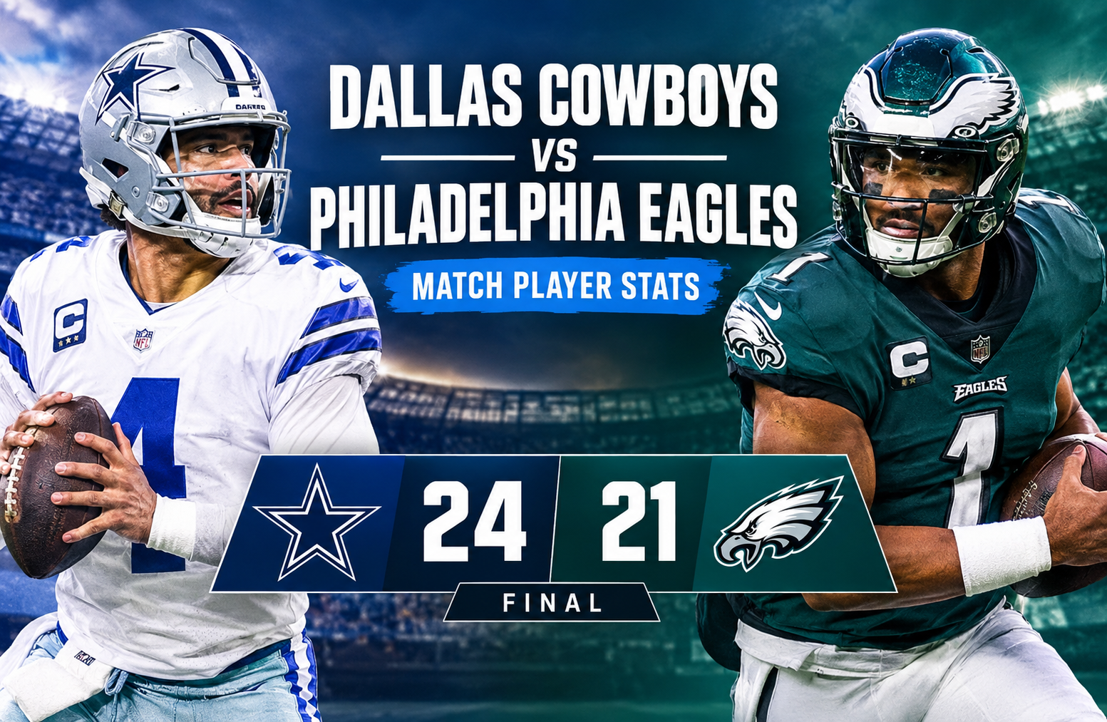
The dallas cowboys vs philadelphia eagles match player stats from November 23, 2025, reveal how Dallas turned a 21-point deficit into a 24-21 victory over Philadelphia. The Cowboys finished with 348 passing yards from Dak Prescott, 146 receiving yards from George Pickens, and 125 rushing yards as a team. Philadelphia started quickly behind Jalen Hurts and A.J. Brown but failed to score after halftime. The final numbers tell a story of contrasting offensive approaches, lost fumbles, defensive adjustments, and a second-half comeback that changed the outcome of this NFC East rivalry.
This breakdown examines the final score, passing and rushing production, receiving performances, defensive contributions, turnovers, special teams, and the statistical differences that explain the result. All player figures below are based on the supplied ESPN box-score data for the November 23 meeting.
Dallas Cowboys vs Philadelphia Eagles Match Player Stats: Game Summary
The game between Dallas and Philadelphia produced two very different halves. The Eagles scored 21 points in the first half, while the Cowboys gradually built momentum and scored 17 unanswered points after halftime.
| Game detail | Result |
| Matchup | Dallas Cowboys vs. Philadelphia Eagles |
| Date | November 23, 2025 |
| Final score | Dallas Cowboys 24, Philadelphia Eagles 21 |
| Venue designation | Dallas home game |
| Eagles record entering the game | 8-3 |
| Cowboys record entering the game | 5-5-1 |
| Dallas passing leader | Dak Prescott |
| Philadelphia passing leader | Jalen Hurts |
| Dallas receiving leader | George Pickens |
| Philadelphia receiving leader | A.J. Brown |
| Dallas rushing leader | Javonte Williams |
| Philadelphia rushing leader | Jalen Hurts |
Dallas won despite trailing 21-7 at halftime. Philadelphia’s offense produced three first-half touchdowns but could not add to its total in the final two quarters.
The difference was not simply the final passing-yard total. Dallas generated more total rushing yards, gained more yards per reception, and converted its passing opportunities into two receiving touchdowns. Philadelphia’s offense remained productive through the air, but its scoring disappeared after the break.
Quarter-by-quarter scoring
| Quarter | Philadelphia Eagles | Dallas Cowboys |
| First quarter | 14 | 0 |
| Second quarter | 7 | 7 |
| Third quarter | 0 | 7 |
| Fourth quarter | 0 | 10 |
| Final score | 21 | 24 |
Philadelphia’s 14-point opening quarter created an early advantage. The Eagles added another touchdown in the second quarter, while Dallas finally found the end zone before halftime.
The third quarter marked a major change. Dallas scored seven points and held Philadelphia scoreless, reducing the deficit to seven. In the fourth quarter, another touchdown and a successful scoring sequence gave the Cowboys the three-point lead they needed.
The key statistical pattern is clear: Philadelphia produced all its points before halftime, while Dallas scored 17 points in the second half. That shift made the final quarter more important than the opening burst.
Dak Prescott vs. Jalen Hurts: Passing Stats Compared
The quarterback comparison highlights two different types of passing production. Prescott delivered more yardage and a higher passer rating, while Hurts completed more passes and avoided an interception.
| Passing statistic | Dak Prescott, DAL | Jalen Hurts, PHI |
| Completions | 23 | 27 |
| Attempts | 36 | 39 |
| Completion percentage | 63.9% | 69.2% |
| Passing yards | 348 | 276 |
| Yards per attempt | 9.8 | 7.4 |
| Passing touchdowns | 2 | 1 |
| Interceptions thrown | 1 | 0 |
| Sacks taken | 1 | 1 |
| Sack yards lost | 6 | 13 |
| Passer rating | 103.2 | 99.2 |
| QBR | 60.6 | 50.5 |
Dak Prescott’s performance
Prescott completed 23 of 36 passes for 348 yards and two passing touchdowns. His 9.8 yards per attempt was the strongest indicator of Dallas’ downfield efficiency.
His completion rate of approximately 63.9% was lower than Hurts’ 69.2%, but Prescott produced 72 more passing yards on three fewer completions. That difference suggests Dallas generated more yardage on its successful throws rather than relying as heavily on shorter completions.
Prescott also recorded one interception. That turnover was a negative mark in an otherwise productive passing performance, but his 103.2 passer rating and 60.6 QBR reflected a strong overall contribution.
One important distinction is that passing yardage alone does not prove that a quarterback played better in every situation. Down, distance, defensive coverage, pressure, and turnover timing all affect a quarterback’s impact. In this game, however, Prescott’s ability to generate explosive receiving production was central to Dallas’ comeback.
Jalen Hurts’ performance
Hurts completed 27 of 39 attempts for 276 yards, one passing touchdown, and no interceptions. His completion percentage was approximately 69.2%, the better mark of the two starting quarterbacks.
Hurts also posted a 99.2 passer rating. His 50.5 QBR was below Prescott’s 60.6, although these are different evaluation systems and should not be treated as interchangeable measurements.
The biggest limitation in Hurts’ passing line was his lower yardage per attempt. At 7.4 yards per attempt, his passing production was less explosive than Prescott’s 9.8. That gap helps explain how Dallas gained more passing yards even though Hurts completed four additional passes.
Hurts was not inefficient in every respect. He protected the ball through the air, completed nearly seven out of every ten attempts, and added two rushing touchdowns. The more important team-level question is why Philadelphia’s offense could not sustain its first-half scoring pace.
What the quarterback comparison tells us
Three details stand out:
- Passing efficiency: Prescott generated more yards per attempt and finished with the higher passer rating.
- Ball security: Hurts avoided interceptions, while Prescott threw one.
- Scoring contribution: Prescott threw two touchdowns, while Hurts threw one and added two on the ground.
The figures show why quarterback analysis should combine passing volume, explosive plays, turnovers, and rushing contributions instead of focusing on completion percentage alone.
Rushing Stats: Javonte Williams Leads Dallas
Dallas established a clear advantage in rushing volume and total production. The Cowboys recorded 125 rushing yards on 31 carries, while Philadelphia finished with 63 yards on 18 carries.
| Rushing statistic | Dallas Cowboys | Philadelphia Eagles |
| Team carries | 31 | 18 |
| Rushing yards | 125 | 63 |
| Yards per carry | 4.0 | 3.5 |
| Rushing touchdowns | 1 | 2 |
| Longest run | 21 yards | 8 yards |
Dallas gained 62 more rushing yards and averaged half a yard more per carry. Philadelphia, however, scored two rushing touchdowns compared with Dallas’ one.
This contrast matters because rushing yardage and rushing touchdowns measure different outcomes. Dallas gained more ground across its attempts, but Philadelphia used Hurts’ mobility to convert rushing opportunities into points.
Javonte Williams’ rushing production
Williams led Dallas with 20 carries for 87 yards, averaging 4.4 yards per attempt. His longest run covered 20 yards, and he did not score a rushing touchdown.
Williams accounted for most of the Cowboys’ conventional rushing workload. His 20 carries represented a substantial portion of Dallas’ 31 team attempts and helped the offense maintain a balanced approach alongside Prescott’s passing attack.
His 4.4 yards per carry exceeded the Dallas team average of 4.0. That difference suggests his individual rushing production was more efficient than the team’s overall figure, which also included quarterback and other player carries.
Williams’ contribution was particularly valuable in a game where Dallas needed to keep moving the chains while gradually erasing a 14-point halftime deficit.
Malik Davis provides a useful change of pace
Davis finished with three carries for 24 yards, averaging 8.0 yards per carry. His longest run was 21 yards.
Although his workload was much smaller than Williams’, Davis delivered a strong per-carry return. His 21-yard run was also the longest rushing play listed for either team.
Small-sample rushing averages require caution. Three attempts cannot establish that a player would maintain an 8.0-yard average with a larger workload. Still, Davis’ production demonstrates the value of a secondary runner who can create yardage when given an opportunity.
Dak Prescott’s rushing contribution
Prescott added five carries for nine yards and one rushing touchdown. His average was 1.8 yards per carry, but the touchdown was more important than the average in terms of scoring.
Quarterback rushing numbers need context. Kneel-downs, scrambles, and designed runs can affect the total, so yards per carry do not always capture the value of a quarterback’s rushing contribution. In this game, Prescott’s rushing touchdown provided a scoring element beyond his two passing touchdowns.
Philadelphia’s rushing attack
Hurts led Philadelphia with seven carries for 33 yards and two rushing touchdowns. He averaged 4.7 yards per carry, with a longest run of eight yards.
Saquon Barkley recorded 10 carries for 22 yards, averaging 2.2 yards per carry. His longest run covered seven yards, and he did not score a rushing touchdown.
Tank Bigsby had one carry for eight yards.
Philadelphia’s running game therefore relied heavily on Hurts for scoring, while Barkley produced limited yardage on his 10 attempts. Barkley’s 2.2-yard average was a notable contrast with Hurts’ 4.7.
The team total of 63 rushing yards was well below Dallas’ 125. Even with two rushing touchdowns, Philadelphia did not generate the same volume of ground production. This became more consequential when its passing offense stopped scoring after halftime.
Receiving Stats: George Pickens and A.J. Brown Lead Their Teams
The receiving numbers provide one of the clearest explanations for Dallas’ passing advantage. George Pickens recorded 146 yards, while Philadelphia’s A.J. Brown led his team with 110.
| Receiving statistic | Dallas Cowboys | Philadelphia Eagles |
| Team receptions | 23 | 27 |
| Team targets | 35 | 36 |
| Receiving yards | 354 | 289 |
| Yards per reception | 15.4 | 10.7 |
| Receiving touchdowns | 2 | 1 |
| Longest reception | 48 yards | 41 yards |
Dallas gained 65 more receiving yards despite recording four fewer receptions. Its 15.4 yards per reception was substantially higher than Philadelphia’s 10.7.
The difference points to a more explosive Dallas passing attack. The Cowboys converted catches into larger chunks of yardage, while Philadelphia recorded more receptions but generated less yardage overall.
George Pickens: Dallas’ leading receiver
Pickens caught nine of nine listed targets for 146 yards and one touchdown. He averaged 16.2 yards per reception, and his longest catch covered 43 yards.
His 146 yards represented a major share of Dallas’ 354 receiving yards. Pickens also matched his target total with his receptions in the supplied data, giving him a 100% catch rate for the game.
A perfect catch rate over nine targets is a notable result, but it should not be treated as a guarantee of repeat performance. Catch rates vary with route depth, coverage, target difficulty, and sample size.
The broader point is that Pickens combined volume with explosive production. He did not merely collect short completions. His 16.2 yards per catch helped Dallas stretch the field and create opportunities for its other receivers.
A.J. Brown: Philadelphia’s top receiving threat
Brown finished with eight receptions for 110 yards and one touchdown on 10 targets. His average was 13.8 yards per catch, and his longest reception was 22 yards.
Brown was Philadelphia’s leading receiver in both catches among the listed leading performers and total receiving yards. He also provided the Eagles with a scoring target during their productive first half.
His 110 yards represented a meaningful contribution, especially in a game where Philadelphia’s offense accumulated 289 receiving yards. However, Brown’s longest catch was 22 yards, substantially shorter than the longest receptions recorded by several Dallas players.
That does not mean Brown lacked impact. Receiving value includes touchdowns, first downs, route execution, and defensive attention, not just the distance of the longest play. His production was strong, but Dallas generated more explosive yardage through its receiving group.
CeeDee Lamb adds another downfield option
Lamb caught four passes for 75 yards on 11 targets. His 18.8 yards per reception was higher than Pickens’ average, and his longest catch went for 48 yards.
Lamb’s target volume was significant even though he caught fewer passes than Pickens. Four receptions from 11 targets produces a catch rate of approximately 36.4%, a low figure that deserves context rather than an automatic judgment about his performance.
The 48-yard longest reception shows that Lamb still contributed a major explosive play. A receiver can create substantial yardage from a limited number of completions, particularly when a small number of catches cover large distances.
Jake Ferguson’s contribution
Ferguson recorded five receptions for 60 yards on six targets, averaging 12.0 yards per catch. His longest reception was 19 yards.
His reliable short-to-intermediate production gave Prescott another option beyond the wide receivers. Ferguson also recorded a rushing attempt for one yard, although that carry had little effect on Dallas’ overall rushing total.
KaVontae Turpin creates a big play
Turpin caught one pass for 48 yards on two targets. His single reception matched Lamb’s longest catch and gave Dallas another source of explosive passing production.
A 48-yard reception from one catch produces an eye-catching average, but the small sample matters. It is better interpreted as evidence of one major play than as a stable measure of his receiving efficiency.
Turpin also contributed on special teams, recording three kick returns for 85 yards. His combined involvement in the passing and return games made him a useful source of field-position and explosive-play potential.
Philadelphia’s supporting receivers
Beyond Brown, several Eagles contributed meaningful yardage:
- DeVonta Smith: Six receptions for 89 yards on 11 targets, averaging 14.8 yards per catch. His longest reception was 41 yards.
- Saquon Barkley: Seven receptions for 52 yards on eight targets, averaging 7.4 yards per catch.
- Dallas Goedert: Two receptions for 20 yards on two targets.
- Grant Calcaterra: One reception for eight yards on one target.
- Darius Cooper: Two receptions for seven yards on two targets.
- Xavier Gipson: One reception for three yards on one target.
Smith’s 89 yards were especially notable because his longest catch covered 41 yards. Philadelphia had the ability to generate explosive passing plays, but it did not translate that production into second-half scoring.
Barkley’s seven receptions also show that his offensive role extended beyond rushing. His 52 receiving yards added an important dimension to his total contribution even though his rushing average was low.
Defensive Stats: Tackles, Sacks, and Turnover Opportunities
Defensive box-score figures help explain individual workloads, but they do not tell the entire story of a defense’s performance. Tackles indicate involvement, sacks show certain forms of pressure, and passes defended record disruption of throws. None of these numbers alone measures every contribution to a stop or a change in possession.
| Defensive statistic | Philadelphia Eagles | Dallas Cowboys |
| Total tackles | 70 | 59 |
| Solo tackles | 36 | 35 |
| Sacks | 1 | 1 |
| Tackles for loss | 2 | 2 |
| Passes defended | 4 | 3 |
| Quarterback hits | 6 | 6 |
| Defensive touchdowns | 0 | 0 |
Philadelphia recorded more total tackles and one additional pass defended. Both teams finished with one sack, two tackles for loss, and six quarterback hits.
These figures suggest that both defenses generated some disruption, but neither produced a large sack advantage. Dallas’ comeback should not be attributed to sack totals alone. The final result reflected a combination of offensive execution, turnovers, and Philadelphia’s inability to score in the second half.
Zack Baun leads Philadelphia’s tackle count
Baun recorded nine total tackles, including three solo tackles, and one pass defended. He did not record a sack, tackle for loss, quarterback hit, or defensive touchdown.
His nine tackles led the individual defensive figures supplied for Philadelphia. That workload indicates regular involvement in stopping Dallas’ offensive plays, although tackle totals alone cannot determine how effectively a defender performed on every snap.
Reed Blankenship contributes in coverage
Blankenship recorded eight total tackles, three solo tackles, and one pass defended. He also registered one interception, making him an important figure in the turnover statistics.
An interception is a high-impact defensive event because it ends the opponent’s possession and gives the intercepting team a chance to gain the ball. Blankenship’s interception was the only interception recorded by Philadelphia in the supplied data.
Cooper DeJean and Nakobe Dean
DeJean finished with seven total tackles, five solo tackles, and one pass defended. Dean recorded five tackles, two solo tackles, one sack, one tackle for loss, and one quarterback hit.
Dean’s sack was Philadelphia’s only recorded sack. His combination of a sack, a tackle for loss, and a quarterback hit shows several forms of direct disruption in the box score.
Dallas defensive contributors
Reddy Steward led the listed Dallas defenders with six total tackles, including three solo tackles. Donovan Wilson recorded five tackles, all solo, and one pass defended.
Osa Odighizuwa finished with four total tackles, two solo tackles, one sack, one tackle for loss, and four quarterback hits. His four quarterback hits were particularly notable because they accounted for a substantial portion of Dallas’ six total hits.
Odighizuwa’s pressure production offers a useful reminder that sacks are only one measure of defensive-line effectiveness. Quarterback hits can indicate disruption even when a play does not end in a sack, although the precise effect depends on the timing and result of each play.
Turnovers and Fumbles: A Critical Part of the Result
Turnover statistics require careful interpretation because not every fumble results in a change of possession. The supplied box score lists two team fumbles for each side, but the number lost differs.
| Turnover statistic | Philadelphia Eagles | Dallas Cowboys |
| Team fumbles | 2 | 2 |
| Fumbles lost | 2 | 1 |
| Fumbles recovered | 1 | 2 |
| Interceptions thrown | 0 | 1 |
| Interceptions recorded | 1 | 0 |
Philadelphia lost both of its recorded fumbles, while Dallas lost one. Dallas also threw one interception, and Philadelphia recorded one interception.
The figures show why turnover analysis should separate fumbles from fumbles lost. A team can put the ball on the ground without necessarily surrendering possession. The lost-fumble column is the more direct measure of how often a fumble changed possession.
There is also a distinction between a team’s offensive turnovers and its defensive recoveries. The supplied team totals list Philadelphia with two fumbles lost and one recovery, while Dallas had one fumble lost and two recoveries. These are box-score categories and should not be treated as a complete description of every possession without the play-by-play sequence.
Philadelphia’s fumble issues
Saquon Barkley and Xavier Gipson each recorded one fumble lost. These lost possessions were costly because Philadelphia was unable to add any points after halftime.
The timing of turnovers can matter as much as their number. A turnover that stops a promising scoring drive or gives an opponent a short field may have more immediate consequences than one that occurs far from the end zone. The aggregate figures alone do not establish the exact impact of each fumble, but they identify ball security as an important area to examine.
Dallas also made mistakes
Turpin recorded one fumble lost, while Ferguson recorded one fumble that was not lost. The team also recorded an interception thrown by Prescott.
Dallas therefore did not win by playing a mistake-free game. Instead, it overcame its own turnover and combined greater passing explosiveness with stronger second-half scoring.
This distinction matters when evaluating the result. A comeback does not necessarily mean one team executed perfectly. It means the winning team produced the better final outcome despite the mistakes recorded during the game.
Special Teams: Kicking, Punting, and Returns
Special teams influence field position and scoring opportunities, even when they do not produce a touchdown. The supplied numbers show productive punting from both sides, different kick-return totals, and missed field-goal opportunities.
| Special teams category | Dallas Cowboys | Philadelphia Eagles |
| Kicker | Brandon Aubrey | Jake Elliott |
| Field goals | 1 of 2 | 0 of 1 |
| Extra points | 3 of 3 | 3 of 3 |
| Total kicking points | 6 | 3 |
| Punter | Bryan Anger | Braden Mann |
| Punts | 3 | 5 |
| Average punt distance | 56.0 yards | 50.0 yards |
| Longest punt | 62 yards | 58 yards |
| Punts inside the 20 | 1 | 3 |
Brandon Aubrey and Jake Elliott
Aubrey made one of two field-goal attempts, with a longest successful field goal of 42 yards. He converted all three extra points and scored six kicking points.
Elliott went zero for one on field goals and converted all three extra points, scoring three points. Neither kicker was perfect on field goals, but Aubrey’s successful attempt gave Dallas an additional three points from that category.
The supplied figures list Aubrey’s field-goal percentage at 50% and Elliott’s at 0%. With only two and one attempts respectively, these percentages reflect very small samples and should not be used to draw broad conclusions about either kicker’s overall ability.
Punting and field position
Anger averaged 56.0 yards across three punts, while Mann averaged 50.0 yards across five. Anger’s longest punt covered 62 yards, and Mann’s longest was 58 yards.
Philadelphia recorded three punts inside the 20-yard line, compared with Dallas’ one. That statistic measures placement near the opponent’s end zone, rather than total punt distance alone.
The higher number of Philadelphia punts is consistent with the offense having more possessions that ended without scoring, particularly after halftime. However, the punting figures do not independently establish why each drive ended.
Kick and punt returns
Will Shipley recorded four kick returns for 106 yards, averaging 26.5 yards per return. His longest return covered 30 yards.
Turpin returned three kicks for 85 yards, averaging 28.3 yards per return, with a longest return of 33 yards. He also recorded two punt returns for one yard in total.
Gipson returned two punts for 19 yards, averaging 9.5 yards per return, with a longest return of 14 yards.
These numbers suggest that both teams had opportunities to influence field position through returns. Dallas’ kick-return average was slightly higher, while Shipley produced the larger total kick-return yardage because he handled one additional return.
Team Statistical Comparison: Where Dallas Gained the Advantage
The overall comparison brings the game’s main trends into focus. Dallas gained more passing yards, more rushing yards, and more receiving yards. Philadelphia recorded more completions and receptions, but those additional completions did not produce greater yardage or a higher final score.
| Team statistic | Dallas Cowboys | Philadelphia Eagles |
| Passing yards | 348 | 276 |
| Rushing yards | 125 | 63 |
| Receiving yards | 354 | 289 |
| Passing touchdowns | 2 | 1 |
| Rushing touchdowns | 1 | 2 |
| Total offensive touchdowns | 3 | 3 |
| Interceptions thrown | 1 | 0 |
| Fumbles lost | 1 | 2 |
| Final points | 24 | 21 |
The total offensive touchdown figures are three per team when passing and rushing touchdowns are combined. Dallas’ listed two passing touchdowns and one rushing touchdown equal three, while Philadelphia’s one passing touchdown and two rushing touchdowns also equal three.
The final score difference therefore cannot be explained by offensive touchdown totals alone. Dallas’ additional successful field goal, along with the timing of its scoring, contributed to the three-point margin.
Dallas’ advantage through the air
Prescott’s 348 passing yards exceeded Hurts’ 276 by 72 yards. Dallas also recorded 354 team receiving yards compared with Philadelphia’s 289.
The Cowboys’ 15.4 yards per reception was a key difference. Philadelphia completed more passes, but Dallas extracted more yardage from each catch on average.
This is a useful lesson when reading football box scores: volume and efficiency can point in different directions. More completions can indicate sustained short passing, while fewer receptions can still generate greater total yardage when the offense creates bigger plays.
Dallas’ advantage on the ground
Dallas recorded 125 rushing yards, more than Philadelphia’s 63. Williams’ 87 yards formed the largest individual rushing contribution in the game.
Philadelphia’s rushing touchdowns kept its scoring total competitive, but the lower team rushing output limited its overall ground production. Dallas was able to pair its passing game with a more productive rushing attack.
The turnover difference
Philadelphia lost two fumbles, while Dallas lost one. Dallas also threw an interception, so the turnover picture was not one-sided in every category.
The more useful comparison is that Philadelphia’s two lost fumbles represented additional possessions surrendered. Combined with a scoreless second half, those turnovers form part of the explanation for why the Eagles could not protect their early lead.
The second-half scoring difference
Dallas scored 17 points after halftime, while Philadelphia scored none. This is the most direct statistical description of the comeback.
The figures establish what happened, though they do not by themselves identify every coaching adjustment, coverage change, or play-calling decision that caused the shift. Those details require the full play-by-play record and film review.
Why Dallas Won: Five Statistical Takeaways
1. Prescott generated more explosive passing yardage
Prescott’s 9.8 yards per attempt was significantly higher than Hurts’ 7.4. He also finished with 348 passing yards and two passing touchdowns.
Dallas did not need a higher completion percentage to create more passing production. Its ability to generate larger gains helped it overcome the early deficit.
2. Pickens delivered the leading receiving performance
Pickens finished with 146 yards and one touchdown. His nine catches provided Dallas with a consistent source of yardage and scoring production.
His performance, combined with Lamb’s 75 yards and Turpin’s 48-yard catch, gave Prescott several ways to attack the Philadelphia defense.
3. Williams helped balance the offense
Williams’ 87 rushing yards on 20 carries gave Dallas a reliable ground-game contribution. The Cowboys’ 125 team rushing yards exceeded Philadelphia’s total by 62.
A productive rushing game can help an offense avoid depending entirely on passing. It can also give a team more options when protecting a lead or trying to control the pace of a comeback.
4. Philadelphia’s offense stopped scoring
The Eagles scored 21 first-half points but finished with the same total. Hurts and Brown produced strong individual statistics, yet the team did not score in either of the final two quarters.
The contrast between individual production and team results is important. A quarterback can complete a high percentage of passes, and a receiver can gain more than 100 yards, without the offense maintaining scoring consistency across four quarters.
5. Field goals and turnover management mattered
Dallas converted one of its two field-goal attempts, while Philadelphia missed its only attempt. Dallas also lost fewer fumbles, although it threw one interception.
A three-point game can turn on several small differences. In this case, the field-goal comparison, turnover categories, and second-half scoring all help explain the final margin without suggesting that one statistic alone decided the contest.
How to Interpret Player Stats Without Misreading the Game
Box scores are valuable because they make player production easy to compare. They can also create misleading impressions when numbers are read without context.
A sound approach uses several layers of evidence.
Start with volume. Attempts, carries, targets, and snaps help establish how much responsibility a player received. Williams’ 20 carries, for example, show a larger rushing workload than Davis’ three.
Then examine efficiency. Yards per attempt, yards per carry, and yards per reception help explain how much production came from each opportunity. Prescott’s 9.8 yards per pass attempt is more informative when paired with his total yardage and touchdowns.
Look at scoring contribution. Touchdowns and field goals determine points directly, but they do not capture every useful play. Hurts’ two rushing touchdowns made him a major scoring contributor even though Prescott led the passing comparison.
Account for turnovers. Interceptions and lost fumbles can change possession and erase promising drives. Their significance depends on when they happen and what the opponent does afterward.
Consider the game situation. A team that trails by two touchdowns may throw more often than a team protecting a lead. Similarly, a receiver’s target total may rise when the offense is trying to catch up. Raw totals should be interpreted alongside the score and the timing of production.
Finally, separate verified figures from explanations. The box score confirms yardage, touchdowns, tackles, and turnovers. Claims about defensive adjustments, route design, or coaching decisions require additional evidence from film or play-by-play data. Keeping that distinction clear makes statistical analysis more trustworthy.
Frequently Asked Questions
1. What was the final score of the Dallas Cowboys vs. Philadelphia Eagles game on November 23, 2025?
The Dallas Cowboys defeated the Philadelphia Eagles 24-21. Philadelphia led 21-7 at halftime, but Dallas scored 17 unanswered points in the second half.
2. Who had the most passing yards in the game?
Dak Prescott led both quarterbacks with 348 passing yards on 23 completions from 36 attempts. Jalen Hurts recorded 276 passing yards on 27 completions from 39 attempts.
3. Who was the leading receiver for each team?
George Pickens led Dallas with nine receptions for 146 yards and one touchdown. A.J. Brown led Philadelphia with eight receptions for 110 yards and one touchdown.
4. Which player led the game in rushing yards?
Javonte Williams led all listed rushers with 87 yards on 20 carries for Dallas. Jalen Hurts led Philadelphia with 33 rushing yards and two rushing touchdowns.
5. How many turnovers did each team lose?
Philadelphia lost two fumbles and threw no interceptions. Dallas lost one fumble and threw one interception. These figures distinguish lost fumbles from all recorded fumbles.
6. What was the biggest statistical difference between the teams?
Dallas recorded 348 passing yards and 125 rushing yards, compared with Philadelphia’s 276 passing yards and 63 rushing yards. Dallas also scored 17 second-half points while Philadelphia was held scoreless after halftime.
Conclusion
The Dallas Cowboys’ 24-21 victory over the Philadelphia Eagles on November 23, 2025, was defined by a dramatic change in scoring momentum. Philadelphia built a 21-7 halftime lead, but Dallas responded with 17 unanswered points to complete the comeback.
Dak Prescott’s 348 passing yards and two passing touchdowns gave Dallas an advantage through the air, while George Pickens’ 146 receiving yards supplied the game’s leading receiving performance. Javonte Williams added 87 rushing yards, helping the Cowboys finish with 125 team rushing yards.
Philadelphia had its own strong individual performances. Hurts threw for 276 yards without an interception and scored twice on the ground, while Brown collected 110 receiving yards and a touchdown. However, the Eagles could not turn their first-half production into additional points after the break.
The most revealing figures are the difference in passing yardage, Dallas’ advantage on the ground, the fumble totals, and the 17-0 second-half scoring margin. Together, they explain the result more clearly than any single player’s statistics. The game also demonstrates why accurate football analysis should consider volume, efficiency, turnovers, and scoring context together rather than relying on one headline number.
For readers examining the dallas cowboys vs philadelphia eagles match player stats, the central lesson is that early dominance does not guarantee a win. Dallas generated more explosive passing production, maintained a stronger rushing total, and finished its scoring opportunities more effectively over the final two quarters.